Things Look Pretty Flat


Click to Enlarge
 Mass and Schwarzschild Radii of Various Celestial Objects:*
 Object Mass RSchwarzschild
 Neutron Star 2.8 × 1030 kg 4.2 × 10³ m = 4.2 km
 Sun 2.0 × 1030 kg 3.0 × 10³ m = 3 km
 Jupiter 1.9 × 1027 kg 2.2 m = 2.2 m
 Earth 6.0 × 1024 kg 8.7 × 10⁻³ m = 8.7 mm
 Moon 7.3 × 10²² kg 1.1 × 10⁻⁴ m = 0.11 mm !

https://astronomy.swin.edu.au/cosmos/S/Schwarzschild+Radius

“When formal observations begin in July, DKIST, with its 13-foot mirror, will be the most powerful solar telescope in the world. Located on Haleakalā (the tallest summit on Maui), the telescope will be able to observe structures on the surface of the sun as small as 18.5 miles (30 kilometers). This resolution is over five times better than that of DKIST’s predecessor, the Richard B. Dunn Solar Telescope in New Mexico.”

— Neel V. Patel, MIT Technology Review


The Projection Geometry of a Theoretical Net-Zero Gravitational Field

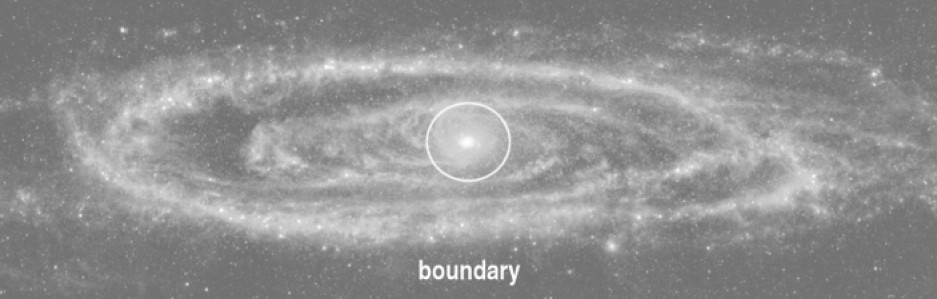
There are some equations I’m working on.[1]  They are intended to describe a projection from the outside surface of a sphere to the inside surface of a concentric spherical shell. This paradigm corresponds to a hypothetical gravitational field that has a net zero gravitational force in a universe with a single black hole.[2]

In two dimensions, the equations are scaled and rotated logarithmic spirals, which preserve the angles between its tangent and the intersecting circle — the polar slope angle is constant, which is consistent with flat planar projections. The equations in three dimensions will be published in a later post.


There exists at least one r11) and a scaled inverse r21 + φ2), where every product of r1(φ) with r2 (φ) is constant. See the proof at the bottom of the page. 

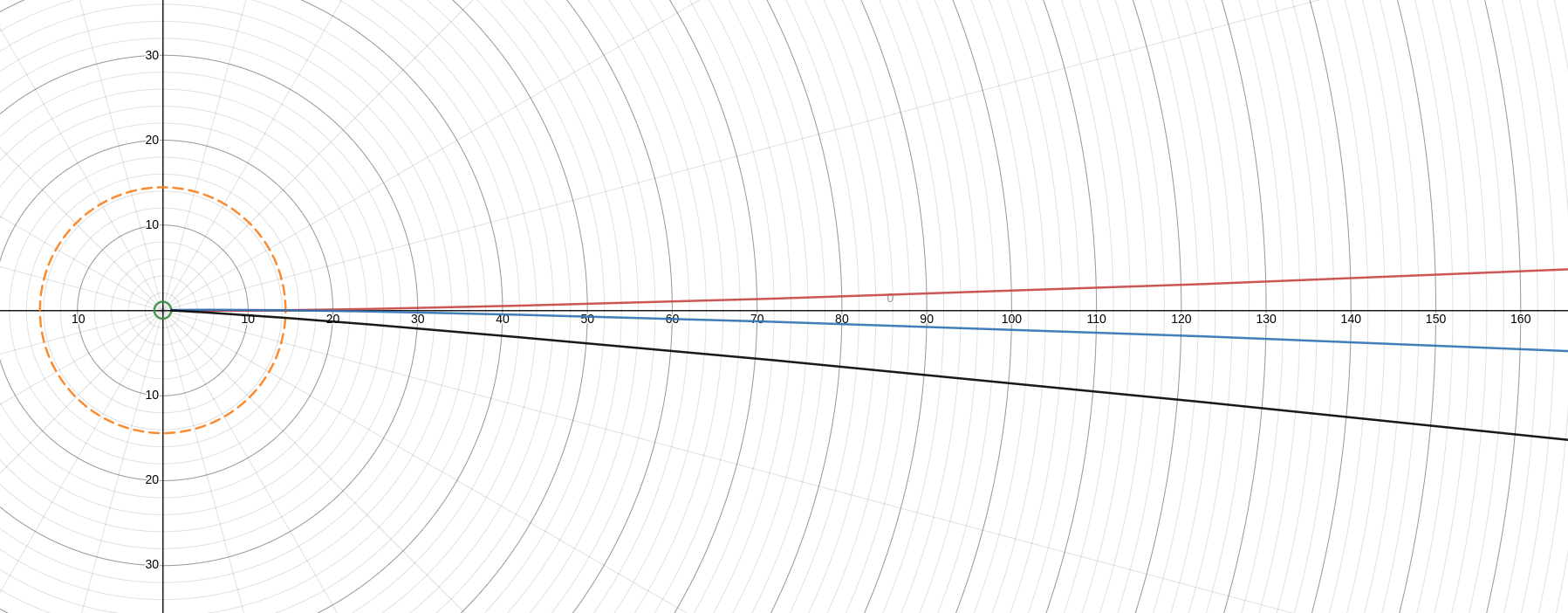
See equations (1-5) below, which include:
  (1) logarithmic spiral in polar form (red),  
  (2) the inverse of equation 1 (black),  
  (3) equation 2 scaled and rotated (blue), and  
  (4) domain, scaling and rotational factors.

\begin{flushleft}
\begin{small}
{r_a = 1,  \quad r_b = 2, \quad r_c = 4} \quad : \quad {r_b^2 = r_a \cdot r_c}
\end{flushleft}


(1)   \begin{equation*} $ ${r(\varphi) = b \cdot e^{\frac{k}{\pi} (\varphi)}}$ \end{equation*}

(2)   \begin{equation*} $ $r(\varphi) = \frac{1}{b} \cdot e^{-\frac{k}{\pi}(\varphi)$ \end{equation*}

(3)   \begin{equation*} $ $r(\varphi) = b \cdot e^k \cdot e^{-\frac{k}{\pi} (\varphi+\pi)}= b \cdot e^{-\frac{k}{\pi} (\varphi)}}$ \end{equation*}

(4)   \begin{equation*} $ $-\frac{\pi \cdot \ln{b}}{k} \leq \varphi \leq \frac{\pi \cdot \ln{b}}{k} $ \end{equation*}

(5)   \begin{equation*} $ $k = P^{-1} \ln{b} $ \end{equation*}

The variable P is the subtended projection angle in units of turns, 1=π (or 1=1/2 turn), and the variable b is the radius of the neutral surface, where all projection lines meet.


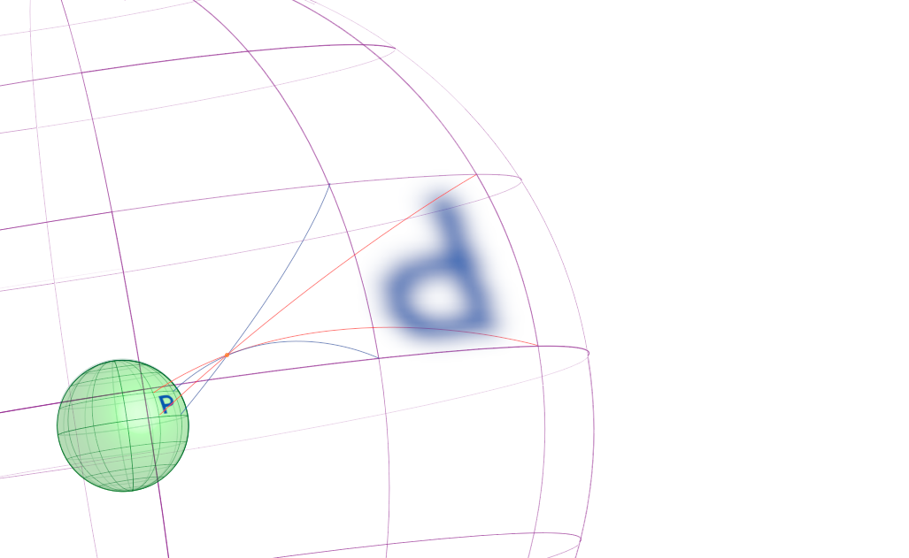
Below is an example drawn to represent the projection in three dimensions (not to scale) in a universe containing only a single black hole — a very small universe with a very large black hole!
[Click the image to enlarge.]

[1] For a more dynamic view of these equations, visit desmos.com.
[2] Here is where I am on all this speculation. Click the link to see a recently reported-measurable experiment inside (see page 18). This link has a graphic on page 24 that might be helpful.

Happy Pi Day, everyone!


PROOF:\begin{flushleft*}

    \begin{align*} b \cdot e^k \cdot e^{-\frac{k}{\pi} (\varphi+\pi)}  \quad \times \quad {b \cdot e^{\frac{k}{\pi} (\varphi)}} \quad &= \quad b^2 \\ e^k \cdot e^{-\frac{k}{\pi} (\varphi+\pi)}  \quad \times \quad {e^{\frac{k}{\pi} (\varphi)}}\quad &= \quad 1 \\ e^k \cdot e^{-\frac{k}{\pi}(\varphi)-\frac{k}{\pi}(\pi)} \quad \times \quad {e^{\frac{k}{\pi} (\varphi)}}\quad &= \\ e^k \cdot e^{-\frac{k}{\pi} (\varphi)} \cdot e^{-k} \quad \times \quad {e^{\frac{k}{\pi} (\varphi)}}\quad &= \\ e^0 \cdot e^0 \quad &= \\ \end{align*}