The current range of estimates on the quantity of dark matter in the Universe often range from the mid- to upper-90s in percent.

At these quantities, under these large fractions of one, it would be equally plausible to assume that what is being observed (not being observed) is a presence so large that the number could effectively be 100% or inversely, zero (plus or minus three percent).

For example, adding all the matter in the Universe to equal in parts to some form of “dark-matter” would yield this result of zero (or inversely, 100).

It is supported by consensus that such quantities of anti-matter do not exist, and can not exist, in the Universe without interacting with matter and self-annihilating creating visible light and visible energy.

But in what other form could “anti-matter” be comprised?

Could there be a form of dark “anti-matter” that is non-interacting and repulsive of itself and all forms of matter, which is saturating every nominal volume of space unable to interact with any particle, even itself?

These questions are being answered in many ways, rightly or wrongly, using Sting Theory, MOND, and other ideas.

The motivations for these questions and answers are predicated by observations on the rotational dynamics of galaxies: Where they appear non-Keplerian, the gravitational attraction is presumed to be very small.

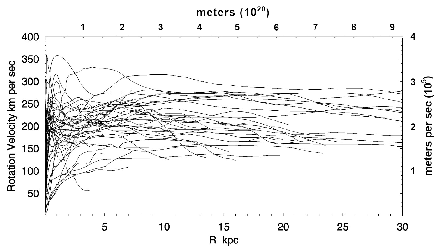
For example, in the image below^[1], one can observe on the left-hand side an area where a “dip” emerges and then rises. This behavior is shared among many of the plots in the image and is indicating motion not consistent with Keplerian celestial orbits.

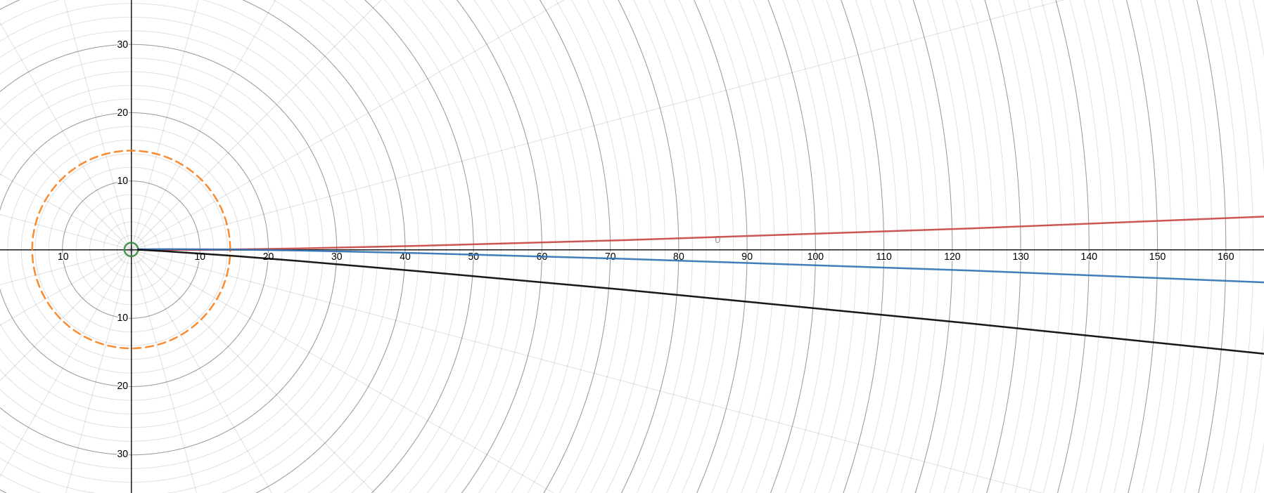
Below, one such area is approximated by shading in yellow within two curves. Similar curves are drawn using other values and colors:

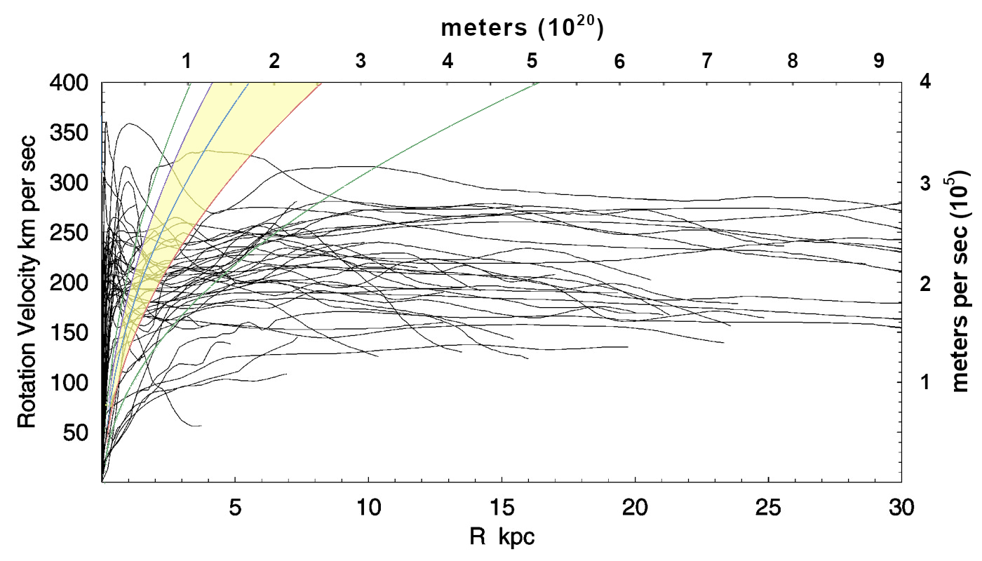
This family of lines are where the rotational velocity squared is divided by the radius and constant.

(1)  

The yellow area is bounded by the violet curve on the left (b = 1.3 x 10^-9 m/sec²), and by the red curve on the right (b = 6.4 x 10^-10 m/sec²). This range of values for b is also highlighted with yellow in the table below.

The value of the green curve on the far left is 1.6 x 10^-9 m/sec². The value of the green curve on the far right, 3.2 x 10^-10 m/sec².

All the values of b are are within or near 10^-9 to 10^-10 in units of m/sec².

This range, plus or minus two orders of magnitude (10^-7– 10^-12 ), is the region of study.

Perhaps certain units of acceleration are within the range of experimentation, given certain devices such as a very long pendulum, or other means.

 

 Values of V²/R

Color of Curve	b (m/sec2)
Green (left)	1.6 x 10-9
Violet	1.3 x 10-9
Blue	1.0 x 10-9
Red	6.4 x 10-10
Green (right)	3.2 x 10-10

 

This website examines one special case, where the lower limit of the gravitational force exists and is within or around this range, such that:

1. All the forces of observable matter in the universe is equal to all the forces of an unobservable dark anti-matter type force, as described here.^[1]

This dark anti-matter type force is repulsive and saturates every nominal volume of space equally. The quantity integrated across vast distances are significant and propel the expansion of the universe.

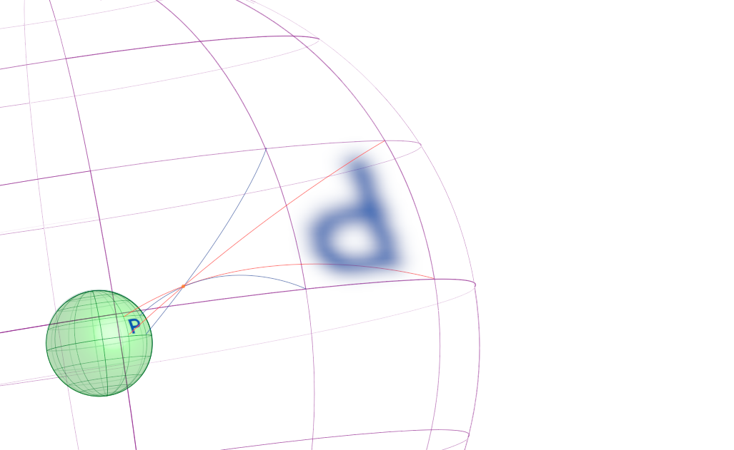
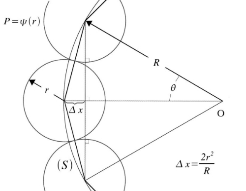
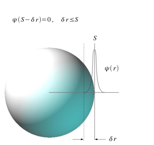
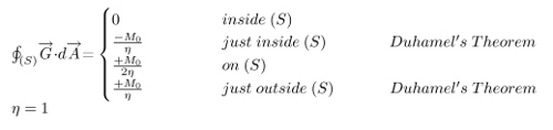
2. So that certain projection mathematics apply, there is an inverse-oriented surface at the limit of the Schwarzschild radius, as described here.^[1][2]

DISCLAIMER: This assessment of the universe is not a consensus among any scientists that I know of. Anything claimed here is hypothetical.

Happy Pi Day, everyone!

The image below represents a super-gravitational Cavendish-like celestial mechanical pendulum laboratory 1 – 10 kilometers below the surface of the Earth that is currently under construction (in my dreams).

It would be interesting for me to learn how such a hanging mass would move, and how much of the swinging motion (and noise) could be brought to a stop (so as to make further measurements). Perhaps the bottom can be cooled with inlet gases being forced out with a Helium Venturi or some other means.

Dampening every bit of noise is critical, like in all these types of submillimeter-scale gravitational experiments.

The torus shape represents a stellarator that is mass producing neutrons (and Helium).

Neutrons are collected and filtered into a beam, which passes through a small crystal attached to the bottom of a 1-kilogram mass. This suspension is isolated from the environment as much as possible.

Images of neutron diffraction patterns (Bragg’s peaks) are taken to measure tiny displacements.

Perhaps the pendulum fiber may be an ultra-high-molecular-weight polyethylene of no more than .05 millimeters in diameter, and according to calculations, weigh less than 3 grams. Perhaps it can be glass.

Theoretic Displacements

Theoretic displacements at the bottom of the 10 kilometer pendulum would be monitored within the order of 1 angstrom or less, ideally.

Forces applied, measured, and monitored, would be on the order of magnitude 10^-11 Newtons plus or minus an exponent in units of free-fall acceleration. See the free body diagram below (not drawn to scale), and download the PDF of calculations.

What is the magnitude of kinematic noise that would be interfering with such an experiment 10 kilometers below the surface of the Earth, flying planes, passing trains, and automobiles? And how vibrations can be mitigated, eliminated.

What would the final results of displacements be with respect to the varying degrees of force, as entered into the table. Would there be any surprises?

• PDF of the free body diagram, a short description, a table of values, and static equilibrium calculations.

Related Content

There are some fun videos of Cavendish-like experiments to watch on YouTube, [1] [2]. And a wonderful documentary on LIGO.

NIST has an awesome webpage describing a 2014 workshop on measuring the Newtonian constant G. Several dozen scientists from around the world participated in the gathering.

And there is this March 2023 paper on measuring gravity with milligram levitated masses that I am currently studying.. The gravitational field strength numbers appear to be very close, in the 6 x 10^-10 (m/sec²) range.

Epilogue

After noticing how linear microscopic displacements become with respect to applied forces, I asked myself (see image below): Given that the mass-density of each of the spheres can be anything (e.g., all different), is there a set of such stable displacements that can exist, or almost perfectly linearly?

To me, this looks impossible (the angles are not necessarily to scale). Perhaps as the more linear curvature at the bottom of the radius, the linear approximation becomes increasingly closer until it reaches some quantum state where the spheres are just bouncing around.

Interfaces of tiny displacements in gravitational fields at quantum scales are continually being investigated.

 

Figure 1: No surface at H(r) = 1

Figure 2: Convex surface at H(r) = 1

Figure 1 is a visual representation of a hole (the Schwarzschild radius, also called the gravitational radius) as a step function, where inside the hole H(r) =1, and outside the hole, which extends to infinity in this example, H(r)=0.

Figure 2 is a visual representation of a sheet intersecting the outer surface of a sphere for comparison.

Figure 3: Concave surface at H(r) = 1

A black hole I prefer to describe by Figure 1, one with no interior surfaces or walls.

The hole is circular at every angle. The images above are an aesthetic representation of a hole in a sheet from an angled perspective, and the angled perspective is used only for emphasis to distinguish the outside surface of a sphere, from the inside surface of a sphere, and a hole with no observable surfaces.

All sorts of things can be happening outside the hole, where H(r) = 0. This is not discussed anywhere here on this blog — on the contrary, there is nothing observable inside the hole, no observable inside surfaces. The only edge is a delta function at the Schwarzschild radius.

Again, inside the hole there are no walls like there is inside a cavity radiator. Furthermore, there are no angles in which the hole can be observed, as implied by the images.

The hole (Schwarzschild radius) is circular at every angle, and by definition radiates nothing. And the hole is not recognized to contain any inside surfaces, such as shown in representations above, and can not be anything else but a hole because there is no reflection nor propagation of light from any observable surfaces.

Nevertheless, an arbitrary surface could be mathematically constructed in a geometrically projected space. There are different ways to graphically represent and rationalize various surfaces with a black hole “surface,” such as projected surfaces, or as the surfaces of projections, and vice versa. But by definition, a black hole is a hole. Just outside the gravitational radius is the observable activity, turbulence, heat, light, etc.

Regardless of these surfaces or no-surfaces details, paths of gravitation in this region are stipulated to be inverted as a result of the geometry as described elsewhere on this blog in detail,¹ its predicate is also discussed, its approximate scale, and where these boundaries may exist,² and how to test for this type of “non-orientability,” whether this inversion exists or not.³

FOOTNOTES:

1. The Projection Geometry of a Theoretical Net-Zero Gravitational Field
2. A Theoretical Net-Zero Gravitational Field
3. Notes on the Black Hole Moon Schwarzschild Radius (0.11 mm) Projection

CORRECTION: An earlier version of this post improperly converted radians to arcseconds, and some table entries were errors, among other errors. [July 28, 2022]

Calculations below provide a demonstration on how using the Rayleigh criterion (R = λ/D) may be used to distinguish between two sources of radiation emitted from the surface of the Moon.  The two sources, which are emitted are: ● 0.11 mm apart ● viewed from a distance of 1.2 AU, and ● to be detected by a 16,000-meter detector.

According to the calculation, the radiation required for proper resolution would be gamma rays of wavelength 9.9 x 10^-6 micrometers (3.0 x 10¹⁹ Hz) , or 124 keV.

The average distance to the Moon from Earth is 385,000 km (385,000,000 m). However, detectors must be farther than b _Moon  =  9 x 10 ¹⁰ m (0.6 AU). 

The distance b _Moon  is described in previous posts as a hypothetical spherical boundary (b) between which negative and positive gravitational accelerations are in the neighborhood of 10^-10 m/sec² and depend on the gravitational object’s Schwarzschild radius (a) and the radius of the observable universe (c), such that b² = ac.

If detectors were placed 16,000 meters apart, located 1.8 x 10¹¹ m (2 · b _Moon = 1.2AU) from the gamma emission source on the Moon, and the image to resolve is 0.11 mm (1.1 x 10^-4), then:

Tan^-1 (1.1 x 10^-4 m/1.8 x 10¹¹ m) = 6.1 x 10^-16 radians = 1.3 x 10^-10 arcseconds

The Rayleigh criterion R (in arcseconds) = 0.21 λ/D, where λ is the wavelength in micrometres and D is the size of the telescope in metres, or the smallest distance between two gamma ray detectors.^[1]

D = 16,000 meters *

R = 1.3 x 10^-10 arcseconds

(1.3 x 10^-10 x 16,000)/0.21  = 9.9 x 10^-6 μm (gamma rays)

                                                  = 9.9 x 10^-6 μm = 3.0 x 10¹⁹ Hz  = 124 keV

*A 16,000 meter detector would be a very large. However, using a large number of smaller detectors spread across a 16,000-meter area and detecting a small fraction of the emissions may be sufficient to form a conclusion.

The resolution can be improved and the size D may be reduced, when used in conjunction with higher energy gamma rays, such as the decay of Technicium-99, which is used in nuclear medicine, has a half-life of six hours and produces 140 keV gamma rays, or Cobalt-60, which emits two gamma rays with energies of 1.17 and 1.33 MeV and has a half-life of 5.27 years.

Similar calculations can be made with respect to the Earth. Here are some preliminary Python scripts used to calculate the experimental parameters relative to the Moon and the Earth. The purpose of this experiment is to test orientability using gamma rays under extraordinary spatial constraints relative to a gravitational field.

Using a Box with Two Small Holes

For example, a box with two very small apertures containing Cobalt-60 emitting 1.1 – 1.3 MeV gamma rays is placed on the surface of the Moon (see image below). The center between the apertures lies on a plane perpendicular to the gravitational field. Emissions radiating from one of the holes would first have to pass through a filter, and the pair of emissions would be of different wavelengths and distinguishable from the point of view of the detectors.

---

The entire speculation is, given high energy photons across large spatial distances, can orientability under the influence of a gravitational field be tested using the Rayleigh Criterion?

---

 Parameters for Three Experimental Apparatus

Location	Distance between Apertures	Distance to Detectors	Required Energy of Gamma Rays
Moon	~ 0.11 mm	~ 1.2 AU	~ 124 keV
Mars	~ 0.9 mm	~ 4 AU	~ 54 keV
Earth	~ 9 mm	~ 13 AU	~ 18 keV

Click here to visit a site on gamma ray detection, NASA’s GLAST Burst Monitor. For a list of comparable scales, see this NASA planet distance chart.

 

 Mass and Schwarzschild Radii of Various Celestial Objects:*

Object	Mass	RSchwarzschild
Neutron Star	2.8 × 1030 kg	4.2 × 103 m	= 4.2 km
Sun	2.0 × 1030 kg	3.0 × 103 m	= 3 km
Jupiter	1.9 × 1027 kg	2.2 m	= 2.2 m
Earth	6.0 × 1024 kg	8.7 × 10-3 m	= 8.7 mm
Moon	7.3 × 1022 kg	1.1 × 10-4 m	= 0.11 mm !

* https://astronomy.swin.edu.au/cosmos/S/Schwarzschild+Radius

“When formal observations begin in July, DKIST, with its 13-foot mirror, will be the most powerful solar telescope in the world. Located on Haleakalā (the tallest summit on Maui), the telescope will be able to observe structures on the surface of the sun as small as 18.5 miles (30 kilometers). This resolution is over five times better than that of DKIST’s predecessor, the Richard B. Dunn Solar Telescope in New Mexico.”

— Neel V. Patel, MIT Technology Review

 

There are some equations I’m working on.^[1]  They are intended to describe a projection from the outside surface of a sphere to the inside surface of a concentric spherical shell. This paradigm corresponds to a hypothetical gravitational field that has a net zero gravitational force in a universe with a single black hole.^[2]

In two dimensions, the equations are scaled and rotated logarithmic spirals, which preserve the angles between its tangent and the intersecting circle — the polar slope angle is constant, which is consistent with flat planar projections. The equations in three dimensions will be published in a later post.

---

There exists at least one r₁(φ₁) and a scaled inverse r₂(φ₁ + φ₂), where every product of r₁(φ) with r₂ (φ) is constant. See the proof at the bottom of the page. 

See equations (1-5) below, which include:
  (1) logarithmic spiral in polar form (red),  
  (2) the inverse of equation 1 (black),  
  (3) equation 2 scaled and rotated (blue), and  
  (4) domain, scaling and rotational factors.

---

(1)  

(2)  

(3)  

(4)  

(5)  

The variable P is the subtended projection angle in units of turns, 1=π (or 1=1/2 turn), and the variable b is the radius of the neutral surface, where all projection lines meet.

---

Below is an example drawn to represent the projection in three dimensions (not to scale) in a universe containing only a single black hole — a very small universe with a very large black hole!
[Click the image to enlarge.]

[1] For a more dynamic view of these equations, visit desmos.com.
[2] Here is where I am on all this speculation. Click the link to see a recently reported-measurable experiment inside (see page 18). This link has a graphic on page 24 that might be helpful.

Happy Pi Day, everyone!

---

PROOF:

   

Fig 1:  dx=2r²/R  [proof]

Without hypothesizing on how such a classical state exists, a possible “confinement argument” is represented by this drawing that shows that for particles P, if they repel, work has to be performed across distance x to exist inside surface (S).

Resistance to compression is a quantum mechanical reaction that violates classical mechanics.

Because there are limits to the energy of “stationary” massive particles, as there are limits to the capacity for a particle to be stationary, defined by Plank’s Constant, I imagine a circumstance at the core of a collapsing neutron star, under such enormous compression at the core, that the capacity of a particle to remain confined at the very center is lost, and propelled outward, and unable to be replaced by another similar particle, for the very same reason, and as the remaining innermost shell of the core continues to be compressed by the increasing pressure of the collapse, a chain reaction ensues, and the star collapses simultaneously from both the outside inward and the inside outward.

How can I construct a plausible mathematical argument that would prove such a collapse takes place, if indeed it does?

Time delay in quantum coherence and tunneling?

Well, maybe in my dreams.  The counter-arguments to hollow black holes would include statements to the effect that the particles would not all necessarily be fundamental particles,  nor that are all of the same type; another counter-argument made might be that certain properties of the bodies to reach such a heightened state of entropy contradicts the possibility of such implicit order in its behavior (coherence).  Or that the observed diameter of existing “black holes” and neutron stars, and the periods of their orbiting celestial objects, rule out their “hollowness.”

It would be possible that the theoretical fundamental particles in question, ie. those that comprise the entirety of the hypothetical surface, may be a particle that changes state with a period. For example, changing from having mass to not having mass, and these flavor changes corresponding to the period, may also correlate its position and direction relative to the surface and any coherence, or tunneling, across the interior of the sphere (or it’s surface): whether on the inside and moving toward the outside, or vice-versa.

Whether the shell of a “hollow black hole” could be high enough in its density to equal in mass a solid sphere of a similar diameter, ie. to within a few orders of magnitude— to within the resolving power of observations required to discriminate black hole from neutron star diameters, and how these diameters correspond to the periods of surrounding orbiting bodies.

Random notes’ quotes:

Einstein: from the point of view in General Relativity that one finds it “appropriate to introduce a tensor T_uv,  ”^[1]  as “It is only the circumstance that we have no sufficient knowledge of the electromagnetic field of concentrated charges that compels us, provisionally, to leave undetermined in presenting the theory [GR], the true form of this tensor.”^[2] And simultaneously,  to “introduce a negative pressure for which there exists no physical justification.” ^[3] the “cosmological constant”.

Fig: The Rotational Inertia of a Point Mass in a Galaxy as Constant

The diagram above describes a pair of conditions that will manifest a constant rotational inertia about the center of a galaxy: 1) the total mass, and 2) the cross-sectional area of the galactic disk are proportional to the radius. A larger version of the diagram is located here.

Net Gravitational Energy = 0

In Standard Cosmology, the motion of matter—such as stars, and planets about stars, and objects about planets—are all moving about the centers of galaxies. These paths are presumed elliptical and are thoroughly examined and well-understood. The orbital motions of galaxies about other galaxies, however, are less understood; less observed, less measured.

I hypothesize that the orbital motions of galaxies about other galaxies include non-planar orbital periods that are very, very large. And if this chaotic motion is to exist over hundreds of billions of Earth years, a chaotic mixing of galaxies in the closed space of the Universe, albeit across the vast spaces would include paths that are not elliptical about a single stationary point, or foci. As an alternative, the paths may resemble more the motion of the turbulent mixing of oceans, such as the Atlantic Conveyor Belt Circulation here on Earth. [2]

I attempt to explain this turbulent mixing of galaxies as the consequence of a hypothesis that is distinct in its character: Perhaps, the total gravitational energy driving the turbulent mixing is gravitationally positive in composition, like that of Einstein’s Cosmological Constant; and opposed equally, by the total negative gravitational energy bound in collections of matter contained in negative fields, as those described by classical gravitational theory.

The principle that makes this circumstance possible (in hypothesis) is asserted by an argument that is based on symmetry and conservation: that the total negative gravitational energy of these bound collections of matter, is equal to the total positive gravitational energy hypothesized to cause the expansion of the Universe, ie. the appearance, by Doppler Shift, as quantified by Hubble’s Law, and other motion.

The Principle of Universe Expansion is not in dispute; the size and rate of expansion will be argued, however.

DEFINITION: Gravitational Equilibrium: Negative Energy (Orbits of Celestial Bodies) + Positive Energy (“Expansion of the Universe”) = Zero. This is the principle by which all the propositions here are characterized.

Definitions:

“Internal motions” are those elliptical orbital motions about centers of matter, such as satellites about planets, planets about stars, and stars within the Galactic Bulge; these motions are driven by negative gravitational energy, are closed and bound.

“External motions” are those driven by a net gravitational energy that is positive in sign (and hypothetical), that are particular to the motions of objects outside a zero boundary. These motions not only include those of particles in the Galactic Disk but also the motions of distant Galaxies with respect to one another: closed and unbound.

—————————————————————————————————–

[1] With respect to galaxies, I postulate that the boundary between predominately internal motions and external ones is the boundary between the Galalctic Bulge and the Galactic Disk; and that every collection of matter has a similar boundary. This principle and its cause, the central focus of my study, is to be examined continually, and throughout, with increasing detail.

[2] The space of the Universe is postulated to be finite and closed; therefore the Turbulent Mixing of Galaxies across the vast spaces of the Universe are motions along paths that are closed. These paths are closed, but these paths are orbits changing in direction that is not always planar, have average radii similar in scale to the radius of the Universe, and traverse across vast timescales.